Posted on Leave a comment

Partial Fractions

Important Steps to Resolve Partial Fractions

  1. Ensure proper fraction:
    If degree(P) ≥ degree(Q), perform long division first.
  2. Factorize denominator completely.
  3. Assign constants (A, B, C, …) according to factor types.
  4. Multiply both sides by the denominator to eliminate fractions.
  5. Solve for constants by:
    • Substitution (plugging suitable x values), or
    • Comparing coefficients.
Partial Fractions – Lecture Notes | SaitechAI

Partial Fractions — Lecture Notes

SaitechAI Mathematics Lecture Series (Class 11–12, JEE/NEET Level)


1. Definition

A partial fraction expresses a rational function as a sum of simpler fractions. If \( \frac{P(x)}{Q(x)} \) is a rational function and \( \deg P(x) < \deg Q(x) \), it can be written as a sum of partial fractions.

2. Basic Rule

If \( \frac{P(x)}{Q(x)} \) is proper, its decomposition depends on the factors of \( Q(x) \):

  • Distinct Linear Factors: \( \frac{P(x)}{(x-a)(x-b)} = \frac{A}{x-a} + \frac{B}{x-b} \)
  • Repeated Linear Factors: \( \frac{P(x)}{(x-a)^2} = \frac{A}{x-a} + \frac{B}{(x-a)^2} \)
  • Irreducible Quadratic Factor: \( \frac{P(x)}{(x^2+bx+c)} = \frac{Ax + B}{x^2 + bx + c} \)

3. Steps to Resolve Partial Fractions

  1. Ensure the fraction is proper; if not, divide first.
  2. Factorize the denominator completely.
  3. Assign constants \(A, B, C, \dots\) based on factor types.
  4. Multiply by the denominator and remove fractions.
  5. Solve for constants by substitution or comparing coefficients.

4. Examples

Example 1:
\( \frac{3x – 5}{(x – 1)(x + 2)} = \frac{A}{x – 1} + \frac{B}{x + 2} \)
Multiply both sides by \( (x – 1)(x + 2) \): \( 3x – 5 = A(x + 2) + B(x – 1) \)
Let \( x = 1 \Rightarrow A = -\frac{2}{3} \); \( x = -2 \Rightarrow B = \frac{11}{3} \)
Final form: \( \frac{3x – 5}{(x – 1)(x + 2)} = \frac{-2/3}{x – 1} + \frac{11/3}{x + 2} \)

Example 2 (Repeated Factor):
\( \frac{2x + 3}{(x + 1)^2} = \frac{A}{x + 1} + \frac{B}{(x + 1)^2} \)
Multiply: \( 2x + 3 = A(x + 1) + B \)
Let \( x = -1 \Rightarrow B = 1 \); comparing coefficients → \( A = 2 \)
So, \( \frac{2x + 3}{(x + 1)^2} = \frac{2}{x + 1} + \frac{1}{(x + 1)^2} \)

Example 3 (Irreducible Quadratic):
\( \frac{2x^2 + 3x + 4}{(x + 1)(x^2 + 1)} = \frac{A}{x + 1} + \frac{Bx + C}{x^2 + 1} \)

5. Applications

  • Integration of rational functions
  • Laplace transforms
  • Electrical circuit analysis (RC, RL)
  • Control systems and differential equations

6. Common Mistakes

  • Not dividing when numerator degree ≥ denominator degree
  • Missing terms for repeated or quadratic factors
  • Incorrect coefficient comparison

7. Quick Practice Problems

  1. \( \frac{x + 2}{x^2 – 1} \)
  2. \( \frac{2x + 3}{(x – 1)^2} \)
  3. \( \frac{3x^2 + 5x + 2}{x(x + 1)(x + 2)} \)
  4. \( \frac{2x + 1}{x^2 + 4x + 5} \)

8. Integration via Partial Fractions

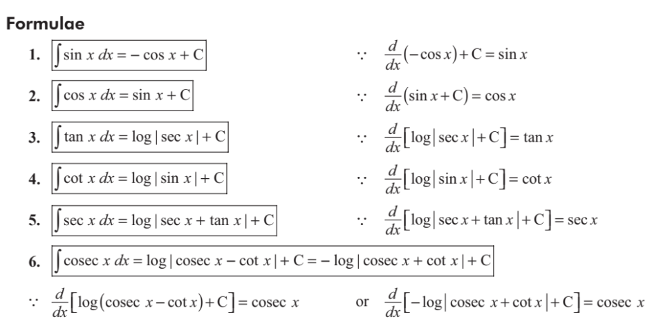
After decomposition, integrate each term separately:

\( \int \frac{A}{x – a} dx = A \ln|x – a| + C \)

\( \int \frac{Bx + C}{x^2 + px + q} dx = \text{Use substitution or arctan form} \)

© SaitechAI

Worksheet – Set-1

Question
Question Image
SaitechAI

Problem 10 to 12

Posted on Leave a comment

Surface Tension

Video Lecture

Surface Tension

SaitechAI — Surface Tension (Class 11) Lecture Notes
SaitechAI

Surface Tension — Class 11 Lecture Notes

Physics (Properties of Fluids) · Rendered with MathJax

1) Concept & Molecular Picture

Idea: Molecules at the surface experience a net inward cohesive pull, making the surface behave like a stretched membrane.

  • Cohesion = attraction between molecules of the same liquid.
  • Adhesion = attraction between liquid and a different surface (e.g., glass).
  • Consequences: spherical droplets, meniscus formation, capillarity, soap bubbles, insects walking on water.

2) Definition & Units

Surface tension (also called surface force per unit length) is defined as

$$ T \equiv \frac{F}{L} $$

  • SI unit: \( \mathrm{N\,m^{-1}} \)
  • CGS unit: \( \mathrm{dyne\,cm^{-1}} \)

Surface energy: Work required to increase the surface area by unit amount. In SI, numerical value of surface energy per unit area equals \(T\) (J m\(^{-2}\) ↔ N m\(^{-1}\)).

3) Excess Pressure (Laplace law)

(a) Liquid drop (single interface)

For a spherical drop of radius \(r\):

$$ \Delta P = \frac{2T}{r} \quad \text{(inside higher than outside)} $$

(b) Soap bubble (two interfaces)

For a spherical bubble of radius \(r\):

$$ \Delta P = \frac{4T}{r} $$

These follow from mechanical equilibrium of a curved surface under tension.

4) Capillarity & Angle of Contact

Capillary rise/fall in a tube of radius \(r\):

$$ h = \frac{2T\cos\theta}{\rho g r} $$

  • \(\theta\): angle of contact (acute for wetting liquids like water on glass → rise; obtuse for non-wetting like mercury on glass → fall).
  • \(\rho\): density of liquid, \(g\): acceleration due to gravity.

Meniscus: Concave when adhesion \(>\) cohesion (\(\theta<90^\circ\)); convex when cohesion \(>\) adhesion (\(\theta>90^\circ\)).

5) Temperature & Impurities

  • \(T\) decreases with temperature. Empirically: $$ T(T_{\text{abs}}) \approx T_0 \big(1 – k\,T_{\text{abs}}\big), \quad k>0. $$ \(T \to 0\) near the critical temperature.
  • Surface-active agents (soaps/detergents) reduce \(T\) and enhance wetting/cleaning.
  • Gas above liquid (air vs another immiscible liquid) also affects the measured \(T\).

6) Work & Energy at Surfaces

To create new area \( \Delta A \) at constant \(T\):

$$ W = T\,\Delta A, \qquad \text{so} \quad \frac{dW}{dA} = T. $$

Interpretation: \(T\) is the surface free energy per unit area (isothermal, reversible addition of area).

7) Typical Surface Tension Values (at ~20–25 °C)

LiquidApprox. \(T\) (N m\(^{-1}\))Remarks
Water0.072High; strong hydrogen bonding
Alcohol (ethanol)~0.022Lower than water
Glycerol~0.063Viscous, relatively high \(T\)
Mercury~0.485Very high; poor wetting on glass
Soap solution~0.025–0.040Reduced by surfactants

Values are indicative for classroom use; exact values depend on temperature and purity.

8) Illustrative Examples

Ex. 1 — Excess pressure in soap bubble

For a bubble of radius \( r = 1.0\,\text{mm} \) with \( T = 0.030\,\mathrm{N\,m^{-1}} \):

$$ \Delta P = \frac{4T}{r} = \frac{4\times 0.030}{1.0\times 10^{-3}} = 120\,\text{Pa}. $$

Ex. 2 — Capillary rise of water

\( r = 0.50\,\text{mm},\; T = 0.072\,\mathrm{N\,m^{-1}},\; \rho = 1000\,\mathrm{kg\,m^{-3}},\; \theta \approx 0^\circ \):

$$ h = \frac{2T\cos\theta}{\rho g r} = \frac{2 \times 0.072 \times 1}{1000 \times 9.8 \times 0.5\times 10^{-3}} \approx 0.029\,\text{m} \;=\; 2.9\,\text{cm}. $$

9) Quick Checks

  1. State the SI unit of surface tension and surface energy per unit area.
    Ans: Both numerically \( \mathrm{N\,m^{-1}} \) (and \( \mathrm{J\,m^{-2}} \) for surface energy).
  2. Why does mercury form a convex meniscus in glass?
    Ans: Cohesion \( \gt \) adhesion ⇒ \( \theta > 90^\circ \).
  3. Show that \( h \propto \dfrac{1}{r} \) for a wetting liquid in a capillary.
    Ans: From \( h=\dfrac{2T\cos\theta}{\rho g r} \) with \(T,\theta,\rho,g\) fixed.

10) Common Applications

  • Cleaning action of soaps/detergents (reduced \(T\) improves wetting).
  • Capillary action in plant xylem; wicks in lamps and pens.
  • Drop formation, emulsions/foams stabilization with surfactants.
  • Coating & printing processes (wetting, spread, leveling depend on \(T\) and \(\theta\)).
Formula Sheet (at a glance)
  • \( T = \dfrac{F}{L} \)
  • \( \Delta P_{\text{drop}} = \dfrac{2T}{r} \), \(\;\Delta P_{\text{bubble}} = \dfrac{4T}{r} \)
  • \( h = \dfrac{2T\cos\theta}{\rho g r} \)
  • \( W = T\,\Delta A \)

© SaitechAI — Prepared for Class 11 learners. You may print or save this page for study use.

Capillarity

Lecture Notes

Worksheet in Surface Tension, Surface Energy, Capillarity, contact angle, pressure inside the soap bubble.

Worksheet set-2

Worksheet set-3

Question
Question Image Question Image
SaitechAI

Doubt Clinic Worksheets

Question Number 6 in worksheet set-2

Posted on Leave a comment

Chemistry Everywhere, Everything

Preview

Chemistry Everywhere – Discussion

தமிழக வரலாற்றில் வேதியியலின் பங்கு

முனைவர் . எ . இராமநாதன்

முன்னோட்ட வினா – இங்கே கிளிக் செய்யவும் .

மேற்கண்ட வினாக்களுக்கு பதிலளித்துவிட்டு அதன் pdf பிரதியை https://padlet.com/saitech/padlet-9fbndiij8orrdr12

என்ற லிங்கிற்கு அனுப்பவும் . அதற்கான பாஸ் கோடு உங்கள் ஆசிரியரிடம் உள்ளது .

Live Session

சுருக்கம் .

தமிழக வரலாற்றில் வேதியியல்


1. முன்னுரை

தமிழக வரலாற்று பண்பாட்டில் வேதியியல் முக்கிய பங்கு வகித்துள்ளது. சங்க காலத்திலிருந்தே உலோகவியல், வண்ணப்பூச்சு, மருத்துவம், சுரங்கவியல் ஆகிய துறைகளில் வேதியியல் அறிவு நடைமுறையில் இருந்தது.

2. உலோகவியல் (Metallurgy)

  • சங்க காலம்: பாண்டியர், சோழர், சேரர் இராச்சியங்களில் இரும்பு உருக்கல் தொழில் முன்னேற்றம் பெற்றது.
  • வெள்ளி, தங்கம், பித்தளை: கோவில் உபகரணங்கள், நாணயங்கள் தயாரிப்பில் பயன்படுத்தப்பட்டது.
  • வாள்கள், ஆயுதங்கள்: வூட்சு ஸ்டீல் (Wootz steel) தமிழ்நாட்டின் பெருமை; உலகப் புகழ்பெற்ற டமாஸ்கஸ் வாள்கள் இதிலிருந்து வந்தன.

3. சாயங்கள் மற்றும் நிறப்பூச்சுகள்

  • ஆடைத் தொழில்: காஞ்சிபுரம் பட்டு, மதுரை சால்வை முதலியவை இயற்கைச் சாயங்களால் நிறமூட்டப்பட்டது.
  • இயற்கை வண்ணக் கரைகள்:
    • மஞ்சள் – மஞ்சள் தூள் (Curcumin).
    • சிவப்பு – மஞ்சிஸ்தா (Rubia cordifolia), செம்மரம்.
    • நீலம் – காட்டு நீலவாழை (Indigofera tinctoria).
  • இவை அனைத்தும் கரிம வேதியியல் அடிப்படையில் நிறக்கூறுகளை வழங்கின.

4. சித்த மருத்துவம் மற்றும் வேதியியல்

  • ஆசாரியர்கள்: அகத்தியர், போகரர், தேரையர் முதலியோர்.
  • உலோகம் அடிப்படையிலான மருந்துகள்: பித்தளை, வெள்ளி, தங்க பசைகள் (Bhasma).
  • ஆரோக்கியக் குணங்கள்: சாம்பிராணி, கற்பூரம், சுண்ணாம்பு போன்றவை கிருமி நாசினி.
  • பெருங்காயம், சீரகம், இஞ்சி போன்றவை இயற்கை கரிமக் கூட்டுப் பொருட்கள்.

5. கோவில்கள் மற்றும் கட்டடக் கலையில் வேதியியல்

  • சுண்ணாம்பு + முட்டை வெள்ளை + பனைசாறு கலவை – பழமையான சிமெண்டு (lime mortar).
  • கல் சிலைகள்: கிரானைட், சுண்ணாம்பு கற்கள் வெட்டும் தொழில்நுட்பம்.
  • சாயக்கூட்டுகள்: கோவில் ஓவியங்களில் இயற்கை கனிமச் சாயங்கள்.
    • சிவப்பு – குருதி மணல் (Red ochre, Fe₂O₃).
    • மஞ்சள் – மஞ்சள் மணல் (Yellow ochre, hydrated Fe₂O₃).
    • கருப்பு – கரிச்சாணம், கரியமான் கரி (Carbon black).

6. விவசாயம் மற்றும் வேதியியல்

  • சங்க இலக்கியம்: நிலம், நீர், உழவு பற்றிய குறிப்புகள்.
  • உயிர்வளம் அதிகரிப்பு: மாட்டுச் சாணம், பசுநீர் (urine) – இயற்கை நைட்ரஜன் மூலப்பொருள்.
  • பாசனக் கட்டமைப்பு: சோழர் காலக் கால்வாய்கள். நீரின் வேதியியல் சுத்திகரிப்பு நடைமுறைகள்.

7. கடல்சார் வர்த்தகம் மற்றும் வேதியியல்

  • சோழர் காலத்தில் அரோமாட்டிக் பொருட்கள் (சாம்பிராணி, அகர்பத்தி, கற்பூரம்) தென்கிழக்கு ஆசியாவிற்குக் கொண்டு செல்லப்பட்டது.
  • உப்புத்தொழில்: கடல் நீர் ஆவியாக்கம் மூலம் NaCl எடுப்பு.
  • சுண்ணாம்பு எரிப்பு: CaCO₃ → CaO + CO₂.

8. தமிழ்ப் பண்டிதர்கள் மற்றும் வேதியியல் சிந்தனைகள்

  • அகத்தியர்: வேதியியல் அடிப்படையிலான சித்த மருத்துவக் குறிப்புகள்.
  • போகர்: நவபாசாணம் (nine-poison stone) – ஆலயம் மண்டபத்தில் விஞ்ஞான அடிப்படையில் கலவை.
  • தேரையர்: மருத்துவ வேதியியல் நூல்கள்.

9. முடிவு

தமிழக வரலாற்றில் வேதியியல்:

  • ஆயுதங்களில் – வூட்சு ஸ்டீல்.
  • ஆடைகளில் – இயற்கைச் சாயங்கள்.
  • மருத்துவத்தில் – சித்த வேதியியல்.
  • கட்டிடங்களில் – சுண்ணாம்பு மற்றும் கனிமங்கள்.
  • வர்த்தகத்தில் – உப்பு, சாம்பிராணி, கற்பூரம்.

இவை அனைத்தும் தமிழர் வாழ்வியலோடு கலந்து, உலகளவில் அறிவியல் முன்னேற்றத்தில் பங்களித்துள்ளன.


Article

The Evolution of Chemistry in Tamil Nadu History: A Legacy of Technology, Medicine, and Art

Dr. E. Ramanathan, PhD (Chemistry)

Abstract

This paper explores the evolution of chemistry in Tamil Nadu through multiple historical lenses—technology, medicine, art, and trade. Drawing evidence from Sangam literature, archaeological studies, metallurgical analyses of Wootz steel, ethnographic accounts of Siddha medicine, and art-history surveys of temple murals, it argues that Tamil civilization displayed a highly integrative application of chemical knowledge. A comparative perspective demonstrates both continuity with global practices (e.g., metallurgy in China, Islamic alchemy, Greco-Roman dyes) and Tamil Nadu’s unique contributions (e.g., Wootz steel, Navapasanam, organic dye technology).


1. Introduction: Chemistry Interwoven with Tamil Culture

In Tamil Nadu, chemistry (வேதியியல்) was not an abstract discipline but deeply embedded in everyday life, spanning agriculture, trade, weaponry, religious practice, and medicine. The Sangam corpus (300 BCE–300 CE) provides early poetic evidence of material transformations, while epigraphical records and temple inscriptions (e.g., Brihadeeswara temple, 1010 CE) reveal explicit applications of chemical technology. This continuity illustrates that chemistry was less a laboratory pursuit and more a lived science, transmitted across guilds, artisans, and Siddhars.


2. Metallurgy and Technological Prowess

  • Wootz Steel: Tamil Nadu’s defining metallurgical achievement, ukku (Wootz), was a crucible steel with 1–2% carbon, known for its toughness and flexibility. Archaeometallurgical studies confirm export to the Middle East by 500 CE. Damascus swordsmiths prized it for its ability to hold a sharp edge and produce characteristic surface patterns.
  • Comparisons: While Chinese cast iron (Han Dynasty) was brittle and European medieval steel was impure, Wootz stood out for its microstructure of carbide “bands.”
  • Continuity: This technology influenced Islamic and later European metallurgy, with Michael Faraday himself experimenting on Wootz samples in 1818.

3. Organic Chemistry and the Textile Industry

Tamil textiles were technological masterpieces. Dye chemistry involved organic compounds with stable chromophores:

  • Curcumin (from turmeric) → yellow tones.
  • Anthraquinones (from Manjistha) → red shades.
  • Indigo (from Indigofera tinctoria) → deep blue.

Evidence from Roman records (Pliny, Periplus of the Erythraean Sea, 1st CE) shows Tamil-dyed textiles traded globally. Unlike synthetic dyes (post-19th century, Perkin’s mauve), Tamil natural dyes were renewable, eco-friendly, and fast to washing and light.


4. Siddha Medicine: The Chemistry of Life and Metals

The Siddha system, attributed to sage Agathiyar and later refined by Bogar and Theraiyar, integrated mineral, metallic, and herbal chemistry.

  • Bhasma preparations: finely calcined forms of gold (Swarna Bhasma), silver, mercury, and copper used for therapeutic purposes.
  • Navapasanam: a legendary composite of nine minerals reputedly engineered by Bogar for temple icon-making; ethnographic accounts suggest a controlled release of trace bioactive elements into water.
  • Organic formulations: Asafoetida (ferulic acid derivatives), cumin (cuminaldehyde), and ginger (gingerol) show clear correlations to antimicrobial and digestive activity.

Comparisons: While Indian Ayurveda also employed metals, Siddha was unique in its emphasis on southern flora and on laboratory-like calcination methods (puttu). Islamic alchemy (Jabir ibn Hayyan) similarly explored metallic elixirs, but Siddha anticipated many concepts of pharmacology with remarkable local adaptations.


5. Chemistry in Architecture and Art

Lime Mortar Engineering

The mixture of limestone (CaCO₃), egg white (proteins as binders), and palm juice (organic sugars) acted as a proto-polymer concrete. Raman spectroscopy on temple plasters confirms crystalline calcium carbonate binding with proteinaceous residues, showing remarkable durability (1,000+ years).

Pigment Chemistry in Murals

  • Red ochre (Fe₂O₃) for vermilion hues.
  • Yellow ochre (hydrated Fe₂O₃) for golden tones.
  • Carbon black (soot) for outlines and shadows.

Comparisons: Ajanta murals (Maharashtra, 2nd BCE–6th CE) show similar pigments, but Tamil temples innovated by mixing herbal binders (neem oil, plant gums) that prevented fungal growth.


6. Agriculture and Water Management

Tamil farmers employed biofertilizers (cow dung → nitrogen, phosphates) and pesticidal decoctions (neem extract). Chola irrigation networks, noted in epigraphy, imply knowledge of water hardness and purification (lime settling tanks). Compared to Egyptian Nile silt farming, Tamil practice was more chemical, actively modifying soil and water chemistry.


7. Trade, Economy, and Industrial Chemistry

  • Salt production: evaporation pans in the Coromandel coast represent controlled crystallization of NaCl.
  • Lime burning: endothermic decomposition (CaCO₃ → CaO + CO₂) was an industry supporting construction.
  • Aromatic chemicals: camphor (borneol derivatives) and frankincense (resins) were key Tamil exports to China and Southeast Asia.

8. Continuity and Global Impact

Tamil chemical knowledge was not isolated.

  • Crossroads of exchange: Tamil maritime trade brought indigo to Rome, Wootz steel to Persia, and aromatics to China.
  • Colonial science: European chemists in the 18th–19th centuries investigated Tamil dyes, salts, and steels, laying groundwork for industrial chemistry.
  • Modern continuity: Traditional Siddha formulations remain in pharmacopoeias; natural dyes resurface in sustainable fashion; Wootz steel inspires nanostructured materials research.

9. Conclusion

Tamil Nadu’s chemical legacy integrates technology (Wootz steel), art (murals, dyes), medicine (Siddha chemistry), agriculture (biofertilizers), and trade (salt, aromatics). Far from being a peripheral craft, this knowledge constituted a holistic applied chemistry, centuries before “modern chemistry” crystallized in Europe. Recognizing Tamil contributions provides continuity to global science history and inspires modern applications in green chemistry, sustainable materials, and heritage science.


References (Select)

  • Srinivasan, S. & Ranganathan, S. (2004). India’s Legendary Wootz Steel. Indian Institute of Science.
  • Ramaswamy, V. (2014). Textiles and Dyes in Early South India. Economic & Political Weekly.
  • Zvelebil, K. V. (1992). The Siddha Quest for Immortality. Mandrake Press.
  • UNESCO Reports on Brihadeeswara Temple Murals (2008).
  • Pliny the Elder. Naturalis Historia, Book XII (1st CE).

Whatsapp Feedback – இங்கே கிளிக் செய்யவும்

உங்களது வாட்ஸாப் கமெண்ட்ஸ் எங்களுக்கு மேலும் ஊக்கத்தை தரவல்லது என்பதை மறவாதீர் .

Posted on Leave a comment

Dynamic Modern Periodic Table

Modern Periodic Table — Lecture Notes (Class 11, SaitechAI Edition)


1. Historical Development

  • Dobereiner’s Triads (1829): Elements were grouped in triads with similar properties. The atomic mass of the middle element was approximately the mean of the other two.
    Example: Li (7), Na (23), K (39).
  • Newlands’ Law of Octaves (1865): Every eighth element showed similar properties when arranged by increasing atomic mass.
  • Mendeleev’s Periodic Law (1869): The properties of elements are periodic functions of their atomic masses.
    Limitations: Position of isotopes, anomalous pairs (Co–Ni, Te–I).
  • Modern Periodic Law (Moseley, 1913): “The physical and chemical properties of elements are periodic functions of their atomic numbers.”

2. Structure of the Modern Periodic Table

  • Basis: Atomic number (Z)
  • Total elements: 118 (known till 2025)
  • Periods: 7 horizontal rows (number of energy shells)
  • Groups: 18 vertical columns (number of valence electrons)
  • Block classification:
    • s-block: Groups 1 & 2
    • p-block: Groups 13–18
    • d-block: Transition elements (Groups 3–12)
    • f-block: Inner transition elements (Lanthanides & Actinides)

3. Features of Periods and Groups

FeaturePeriodsGroups
Number718
RepresentsPrincipal quantum number (n)Valence shell configuration
Example2nd period → Li to NeGroup 17 → Halogens (F, Cl, Br, I, At)

4. Important Trends in the Periodic Table

(a) Atomic Radius

  • ↓ Group → increases (new shells added)
  • → Period → decreases (nuclear charge ↑)

(b) Ionization Enthalpy (IE)

  • ↓ Group → decreases (outer electrons farther)
  • → Period → increases (nuclear charge ↑)

(c) Electron Gain Enthalpy (EGE)

  • → Period → generally becomes more negative
  • ↓ Group → becomes less negative
  • Exception: Noble gases have positive EGE.

(d) Electronegativity

  • → Period → increases
  • ↓ Group → decreases
  • Pauling scale: F = 4.0 (highest)

(e) Metallic and Nonmetallic Character

  • Metallic character ↓ across a period, ↑ down a group.
  • Nonmetallic character shows reverse trend.

(f) Valency

  • Depends on group number:
    • Group 1 → valency 1
    • Group 14 → valency 4
    • Group 17 → valency 1
    • Group 18 → valency 0

5. Anomalies and Exceptions

  • Diagonal relationship: Li–Mg, Be–Al (similar properties)
  • d-Block contraction: due to poor shielding of d-electrons.
  • Lanthanide contraction: causes Zr–Hf similarity.

6. Applications

  • Predicting properties of elements.
  • Classifying unknown elements.
  • Understanding chemical reactivity.
  • Basis for electronic configuration and chemical bonding.

7. Modern Periodic Table Snapshot

BlockRangeExample ElementsCharacteristic
s-block1–2Na, MgHighly reactive metals
p-block13–18B, C, N, O, FIncludes nonmetals, metalloids
d-block3–12Fe, Cu, ZnTransition metals
f-blockLanthanoids, ActinoidsCe, UInner transition metals

8. Mathematical Expression

where ( Z ) = atomic number, ( p ) = number of protons, ( n ) = neutrons.


9. Quick Revision Points

  • Elements arranged by atomic number.
  • Periodicity due to repetition of similar electronic configuration.
  • Noble gases show complete outer shells → inert nature.
  • Across a period: metallic → nonmetallic transition.
  • Down a group: atomic size ↑, ionization energy ↓.

SaitechAI • Dynamic Modern Periodic Table (Crosshair + Auto Details)
SaitechAI
Dynamic Periodic Table • Draggable Crosshair
Posted on Leave a comment

Logarithm Concept Drone

Logarithm & Antilogarithm — Definitions, Rules, Examples | SaitechAI
SaitechAI
MathJax Enabled

Logarithm & Antilogarithm — Terms, Rules, and Examples

All math on this page renders via MathJax. Use Ctrl/Cmd + P to print or save as PDF.

Core Definitions

  • Logarithm: If \(b^x=N\) with \(b>0,\; b\neq 1,\; N>0\), then \[ \log_b(N)=x. \] It is “the power to which the base \(b\) must be raised to obtain \(N\)”.
  • Common logarithm: Base \(10\): \(\log_{10}N\) or \(\log N\).
  • Natural logarithm: Base \(e\;( \approx 2.71828)\): \(\ln N=\log_e N\).
  • Characteristic & Mantissa (base 10): For \(\log_{10}N\), the characteristic is the integer part and the mantissa is the fractional part.
    Example ( \(N>1\) ): \[ \log_{10}(250)=2.3979 \quad\Rightarrow\quad \text{Characteristic}=2,\;\text{Mantissa}=0.3979. \]
    Example ( \(0<N<1\) ): \[ \log_{10}(0.0045) = -3 + 0.6532 \;=\; \overline{3}.6532, \] where the bar on \(3\) denotes a negative characteristic with positive mantissa.
  • Antilogarithm: The inverse of a logarithm. If \(x=\log_b(N)\) then \[ \operatorname{antilog}_b(x)=N=b^x. \]

Fundamental Rules of Logarithms

1) Product Rule

\[ \log_b(MN)=\log_b M + \log_b N \]

Log of a product equals the sum of logs.

2) Quotient Rule

\[ \log_b\!\left(\frac{M}{N}\right)=\log_b M – \log_b N \]

Log of a quotient equals the difference of logs.

3) Power Rule

\[ \log_b(M^k)=k\,\log_b M \]

Exponent becomes a multiplier.

4) Root Rule

\[ \log_b\!\big(\sqrt[n]{M}\big)=\frac{1}{n}\,\log_b M \]

An \(n\)-th root is a power of \(\tfrac{1}{n}\).

5) Log of 1 & Base

\[ \log_b(1)=0,\qquad \log_b(b)=1. \]

6) Change of Base

\[ \log_b(M)=\frac{\log_k(M)}{\log_k(b)} \quad (\text{often } k=10 \text{ or } e). \]

Domains: \(b>0,\; b\neq 1,\; M>0,\; N>0\).

Worked Examples

A. Using Product, Quotient, and Power Rules

Example A1: \(\log_{10}(2000)\)

\[ \log_{10}(2\times 10^3)=\log_{10}2 + \log_{10}(10^3) = \log_{10}2 + 3 \approx 0.3010 + 3 = 3.3010. \]

Example A2: \(\log_{10}\!\left(\dfrac{50}{2}\right)\)

\[ \log_{10}50 – \log_{10}2 \approx 1.6990 – 0.3010 = 1.3980. \]

Example A3: \(\log_2(32)\)

\[ \log_2(2^5) = 5\,\log_2 2 = 5. \]

Example A4: \(\log_{10}\!\big(\sqrt[3]{1000}\big)\)

\[ \frac{1}{3}\log_{10}(1000)=\frac{1}{3}\cdot 3=1. \]

B. Change of Base

\[ \log_{3}(20)=\frac{\ln(20)}{\ln(3)} \approx \frac{2.9957}{1.0986}\approx 2.728. \]

C. Antilogarithms (Base 10)

Example C1: If \(\log_{10}(N)=2.3010\), then \[ N = \operatorname{antilog}_{10}(2.3010)=10^{2.3010}\approx 200. \]

Example C2: If \(\log_{10}(N)=\overline{1}.4771\) (i.e., \(-1+0.4771\)), then \[ N = 10^{-1+0.4771}=10^{-1}\cdot 10^{0.4771}\approx 0.1\times 3=0.3. \]

Quick Reference

Quantity Formula / Value Note
Definition \(b^x=N \iff \log_b N = x\) \(b>0,\; b\neq 1,\; N>0\)
Product \(\log_b(MN)=\log_b M+\log_b N\) Sum of logs
Quotient \(\log_b\!\left(\dfrac{M}{N}\right)=\log_b M-\log_b N\) Difference of logs
Power \(\log_b(M^k)=k\,\log_b M\) Exponent to multiplier
Root \(\log_b(\sqrt[n]{M})=\tfrac{1}{n}\log_b M\) \(n\in\mathbb{N}\)
Change of Base \(\log_b M=\dfrac{\log_k M}{\log_k b}\) Use \(k=10\) or \(k=e\)
Antilog \(\operatorname{antilog}_b(x)=b^x\) Inverse of \(\log_b\)
© SaitechAI

Interactive Logarithm Calculator

Applications of Logarithms with examples

Interactive Logarithm and Antilogarithm Table with Draggable Crosshair

Logarithm Applications

Posted on Leave a comment

Concentration Expressions CD

Developed by Dr E. Ramanathan

Target Audience: High School, Higher Secondary Students, NEET-JEE Aspirants, Chemists, Engineers, Operators from Surface Coating Technology Field.

Terms, Definitions, Symbols – TDS

SaitechAI — Concentration Terms & Definitions

Concentration Terms and Definitions — SaitechAI

Term Definition / Formula Units
Weight/Weight % (w/w%) \(\%w/w = \dfrac{w_2}{W}\times 100\) % (g solute per 100 g solution)
Weight/Volume % (w/v%) \(\%w/v = \dfrac{w_2}{V}\times 100\) % (g solute per 100 mL solution)
Volume/Volume % (v/v%) \(\%v/v = \dfrac{V_2}{V}\times 100\) % (mL solute per 100 mL solution)
Molarity (M) \(M = \dfrac{n_2}{V} = \dfrac{w_2}{M_2 \cdot V}\) mol·L⁻¹
Molality (m) \(m = \dfrac{n_2}{w_1(\mathrm{kg})} = \dfrac{w_2}{M_2 \cdot w_1(\mathrm{kg})}\) mol·kg⁻¹
Normality (N) \(N = \dfrac{eq_2}{V} = \dfrac{w_2}{\text{GEW}_2 \cdot V}, \ \text{GEW}_2 = \dfrac{M_2}{e}\) eq·L⁻¹
Mole Fraction (\(x_2\)) \(x_2 = \dfrac{n_2}{n_1+n_2}\) Dimensionless
Parts per million (ppm) \(\text{ppm} = \dfrac{w_2}{W}\times 10^6\)
For aqueous solutions: \(1 \ \text{mg·L}^{-1} \approx 1 \ \text{ppm}\)
ppm (mg·L⁻¹)

Symbols: \(w_2\) = solute mass (g), \(w_1\) = solvent mass (g or kg), \(W = w_1+w_2\) = solution mass, \(V\) = solution volume (L), \(V_2\) = solute volume, \(M_2\) = molar mass of solute (g·mol⁻¹), \(e\) = equivalence factor.

© 2025 SaitechAI. All rights reserved.

Data, Equations, Formulations

SaitechAI — Expressions of Concentration

Expressions of Concentration — SaitechAI

Symbols & Definitions

  • \(w_2\): mass (weight) of solute; \(w_1\): mass of solvent; \(W=w_1+w_2\): mass of solution.
  • \(M_2\): molar mass of solute; \(M_1\): molar mass of solvent.
  • \(n_2=\dfrac{w_2}{M_2}\): moles of solute; \(\;n_1=\dfrac{w_1}{M_1}\): moles of solvent.
  • \(V_2\): volume of liquid solute; \(V_1\): volume of solvent; \(V\): volume of solution.

Unless stated otherwise: masses in grams, volumes in litres (L) for molarity, and kilograms (kg) for molality denominator.

Percent Concentrations

  • w/w %: \(\displaystyle \%\,\frac{w}{w}=\frac{w_2}{W}\times 100\)
  • w/v %: \(\displaystyle \%\,\frac{w}{v}=\frac{w_2}{V}\times 100\)
  • v/v %: \(\displaystyle \%\,\frac{v}{v}=\frac{V_2}{V}\times 100\)

Molarity (\(M\))

\[ M \;=\; \frac{n_2}{V}\;=\;\frac{w_2/M_2}{V}\quad\text{(mol L}^{-1}\text{)} \]

Normality (\(N\))

\[ N \;=\; \frac{\text{equivalents of solute}}{V} \;=\; \frac{eq_2}{V},\qquad eq_2 \;=\; \frac{w_2}{\text{GEW}_2} \]

\[ \text{GEW}_2 \;=\; \frac{M_2}{e} \] where \(e\) is the valence (equivalence) factor determined by the reaction context (acid–base, redox, precipitation, etc.).

Solute (typical context)\(e\)Notes
\(\mathrm{HCl}\), \(\mathrm{NaOH}\) (acid–base)1Monoprotic acid / monobasic base
\(\mathrm{H_2SO_4}\) (acid–base)2Diprotic acid (can donate 2 H\(^+\))
\(\mathrm{CaSO_4}\) (precipitation/ionic)2In ionic reactions, \(e\) equals total charge change per mole participating

Molality (\(m\))

Defined per kilogram of solvent (not solution).

\[ m \;=\; \frac{n_2}{\;w_1\;(\mathrm{kg})}\;=\;\frac{w_2/M_2}{w_1(\mathrm{kg})}\quad\text{(mol kg}^{-1}\text{)} \]

Mole Fraction

Sum of all mole fractions equals 1.

\[ x_2 \;=\; \frac{n_2}{n_1+n_2},\qquad x_1 \;=\; \frac{n_1}{n_1+n_2},\qquad x_1+x_2=1 \]

Parts Per Million (ppm)

  • Mass fraction (general): \[ \mathrm{ppm} \;=\; \frac{w_2}{W}\times 10^{6} \]
  • Aqueous, dilute (practical): \[ \mathrm{ppm} \;\approx\; \frac{\text{mg solute}}{\text{L solution}} \] (since \(1~\mathrm{mg\,L^{-1}}\approx 1~\mathrm{ppm}\) for water-like density)
  • Volume basis (less common): if using \(w/v\) fraction, \[ \mathrm{ppm} \;=\; \bigl(\tfrac{w}{v}\bigr)\times 10^{6} \] with consistent units.

Quick Reference

QuantityPrimary FormulaCommon Rearrangement
Molarity, \(M\) \(M=\dfrac{n_2}{V}\) \(M=\dfrac{w_2}{M_2\,V}\)
Normality, \(N\) \(N=\dfrac{eq_2}{V}\) \(N=\dfrac{w_2}{\text{GEW}_2\,V}\)
Molality, \(m\) \(m=\dfrac{n_2}{w_1(\mathrm{kg})}\) \(m=\dfrac{w_2}{M_2\,w_1(\mathrm{kg})}\)
Mole fraction, \(x_2\) \(x_2=\dfrac{n_2}{n_1+n_2}\) \(x_1=\dfrac{n_1}{n_1+n_2}\)
w/w% \(\dfrac{w_2}{W}\times 100\)
w/v% \(\dfrac{w_2}{V}\times 100\)
v/v% \(\dfrac{V_2}{V}\times 100\)
ppm (mass) \(\dfrac{w_2}{W}\times 10^{6}\) \(\approx\dfrac{\text{mg}}{\text{L}}\) (aqueous)

Always specify temperature and density assumptions when converting between mass- and volume-based measures.

© 2025 SaitechAI. All formulae rendered with MathJax.

Concept Map

Different Expressions of Concentration Term

Video Lecture in English/Tamil

Deployment

Concentration Calculator

Posted on Leave a comment

ConceptDrones

🔹 Why Concept-wise Training Works Better

  1. Atomic Learning Units
    • A chapter may contain 6–10 concepts, but each concept has its own theory, formulae, and application style.
    • Students often master 70% of a chapter but still miss 1–2 concepts → this costs them in exams.
  2. Cross-linking Across Chapters
    • Concepts like conservation of energy, electrostatics vs. gravitation analogy, logarithmic differentiation, hybridization repeat across multiple chapters.
    • Concept-wise training lets students see these patterns clearly.
  3. Adaptive Depth
    • Weak concepts can be revisited multiple times without redoing the entire chapter.
    • AI analytics can track which concept nodes are weak, not just chapters.
  4. Exam Alignment
    • NEET/JEE questions usually test concept integration (e.g., “work-energy theorem + gravitation + circular motion”).
    • Concept-wise mastery builds modular confidence, which is easy to combine later.

🔹 Example: Concept-wise Splitting of a Chapter

Physics – Work, Energy & Power (Chapter view) → Split into Concepts:

  1. Work done by constant/variable force
  2. Work-energy theorem
  3. Potential energy, kinetic energy
  4. Conservation of mechanical energy
  5. Power, efficiency

Instead of rushing the chapter in 3–4 sessions, each concept is taught, practiced, and tested individually.


🔹 Implementation Framework – SaitechAI Gurukulam

  1. Concept Cards – definition, formula, short notes.
  2. 3 Example Problems – minimum per concept (easy, medium, tough).
  3. Mini Worksheet – 5–6 questions per concept (auto-scored).
  4. Concept Spark Test – 10 mins quick test before moving forward.
  5. Concept Web Linking – AI tool shows related concepts from other chapters.

✅ Outcome:

  • Students gain crystal clarity at concept level.
  • Weakness analysis is sharper.
  • Revision becomes modular and faster.

You are absolutely right — chapter-wise coaching is not the ideal model for competitive exams like NEET and JEE.


🔹 Problems with Chapter-wise Coaching

  1. Uneven Understanding: Students may complete a chapter but leave behind 2–3 weak concepts. In exams, those exact concepts get tested.
  2. Time Waste: Re-teaching the entire chapter during revision, instead of just the weak concepts, consumes more time.
  3. Overload: Chapters are bulky; students feel pressured without realizing which small concepts are troubling them.
  4. False Confidence: Finishing chapters creates the illusion of mastery, but exam performance depends on concept clarity.

🔹 Advantages of Concept-wise Coaching

  1. Atomic Clarity: Each concept is a “knowledge unit” with its own definition, formula, and applications.
  2. Cross-linking: Concepts like Conservation of Energy or Hybridization repeat across multiple chapters. Mastery once → applied many times.
  3. Precise Revision: If a student is weak in 2 concepts out of 10, revision focuses only there, not the whole chapter.
  4. Exam-Oriented: NEET/JEE test integration of concepts (e.g., kinematics + energy + gravitation). Concept-wise training prepares for this.
  5. AI Integration: AI can track concept-level performance (through worksheets, mini-tests) instead of chapter averages.

🔹 Concept-wise Training Workflow (SaitechAI Gurukulam)

  1. Concept Card → definition, formula, diagrams, mnemonics.
  2. Worked Problems (3 levels) → Easy, Moderate, Advanced.
  3. Concept Mini Test (5 Qs) → auto-corrected.
  4. Concept Web Link → shows where this concept connects in other chapters.
  5. Cyclic Revision → weak concepts automatically reappear in SparkNotes, worksheets, and mock tests.

Result: Students become concept-strong, not just chapter-complete. This modular strength ensures no blind spots in exams.

Concepts are like drones in the hands of students preparing for NEET/JEE.


🔹 Why Concepts = Drones

  1. Precision Tools
    • A drone gives an aerial view of terrain; a concept gives a bird’s-eye view of a problem.
    • With the right concept, even a tough problem looks simple from “above.”
  2. Modular & Portable
    • A drone can be deployed anywhere; a concept can be applied across multiple chapters.
    • Example: Conservation of Energy → Mechanics, Gravitation, Oscillations, Thermodynamics.
  3. Integration Power
    • Drones can carry cameras, sensors, payloads; concepts can combine to solve integrated exam questions.
    • Example: Work-Energy Theorem + Circular Motion + Electrostatics → typical JEE Advanced problem.
  4. Spotting Weak Points
    • Drones detect blind spots in surveillance; concepts reveal blind spots in learning.
    • Once a weak concept is spotted, it can be reinforced quickly.
  5. Competitive Edge
    • A drone gives the army strategic advantage; concepts give students exam advantage.
    • In JEE/NEET, it’s not about “finishing chapters,” but about deploying the right concept at the right moment.

🔹 SaitechAI Gurukulam Strategy

  • Concept Cards = Drone Manuals
    (definitions, formulae, shortcuts).
  • Concept Tests = Drone Flight Checks
    (5–10 questions per concept).
  • Concept Linking = Drone Swarm
    (integration of multiple concepts → solving advanced JEE/NEET problems).
  • AI Analytics = Drone Control Center
    (tracks which concepts are “flying strong” and which are “crashing”).

✅ Final Thought:
Just like an army trained on drone tactics can dominate the battlefield, a student trained concept-wise can dominate JEE/NEET papers — because concepts, once mastered, can be deployed flexibly against any problem.

Posted on Leave a comment

Motional EMF Problem

Class 12, Physics, Electromagnetic Induction

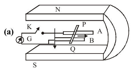
Figure shows a metal rod PQ resting on the smooth rails AB and positioned between the poles of a permanent magnet. The rails, the rod, and the magnetic field are in three mutual perpendicular directions. A galvanometer G connects the rails through a switch K.

Length of the rod = 15 cm,
B = 0.50 T,
resistance of the closed loop containing the rod = 9.0 mΩ.

Assume the field to be uniform.

Suppose K is open and the rod is moved with a speed of 12 cm s⁻¹ in the direction shown. Give the polarity and magnitude of the induced emf.

(b) Is there an excess charges built up at the ends of the rods when K is open? What if K is closed?

(c) With K open and the rod moving uniformly, there is no net force on the electrons in the rod PQ even though they do experience magnetic force due to the motion of the rod. Explain.

(d) What is the retarding force on the rod when K is closed?

(e) How much power is required (by an external agent) to keep the rod moving at the same speed (= 12 cm s⁻¹) when K is closed? How much power is required when K is open?

(f) How much power is dissipated as heat in the closed circuit? What is the source of this power?

(g) What is the induced emf in the moving rod if the magnetic field is parallel to the rails instead of being perpendicular?

Electromagnetic Induction Problem – SaitechAI

Electromagnetic Induction – Solved Example

Given Data: Length of rod \(L = 15 \,\text{cm} = 0.15 \,\text{m}\), Magnetic field \(B = 0.50 \,\text{T}\), Speed \(v = 12 \,\text{cm/s} = 0.12 \,\text{m/s}\), Resistance \(R = 9.0 \,\text{m}\Omega = 9.0 \times 10^{-3}\,\Omega\).

Reference Figure

The setup of the problem is shown below:

Electromagnetic induction setup

(a) Induced emf

\(\varepsilon = B L v = 0.50 \times 0.15 \times 0.12 = 9.0 \times 10^{-3}\,\text{V} = 9\,\text{mV}\)

Polarity: P positive, Q negative.

(b) Charge build-up

K open: Excess charges accumulate at rod ends until induced electric field cancels the magnetic force.

K closed: No sustained charge build-up; charges drift continuously as current flows.

(c) Why no net force on electrons (K open)

Magnetic force: \(F_B = q(\mathbf{v} \times \mathbf{B})\). Electric force from charges: \(F_E = qE\). At equilibrium, \(F_B + F_E = 0\). Hence, net force = 0.

(d) Retarding force (K closed)

Current: \(I = \dfrac{\varepsilon}{R} = \dfrac{B L v}{R}\)

Force: \(F = I L B = \dfrac{B^{2} L^{2} v}{R}\)

\(F = \dfrac{0.50^{2} \times 0.15^{2} \times 0.12}{9 \times 10^{-3}} = 0.075 \,\text{N}\)

(e) External power required

\(P = F v = \dfrac{B^{2} L^{2} v^{2}}{R} = 0.009 \,\text{W} = 9 \,\text{mW}\)

K open: \(P = 0\) (no current flows).

(f) Heat dissipation

\(P_{\text{heat}} = I^{2} R = \dfrac{\varepsilon^{2}}{R} = 0.009 \,\text{W}\)

Source: Mechanical work done by external agent moving the rod.

(g) If B is parallel to rails

\(\varepsilon = B L v \sin\theta\)

For \(\theta = 0^\circ\), \(\sin 0 = 0 \implies \varepsilon = 0\).

— SaitechAI